In a nutshell, keyword extraction is a methodology to automatically detect important words that can be used to represent the text and can be used for topic modeling.
This is a very efficient way to get insights from a huge amount of unstructured text data. Let’s take an example: Online retail portals like Amazon allows users to review products. We want to get insights about a particular product, let’s say a popular smartphone, we may not go through each and every review. Rather, we could use keyword extraction techniques to find reviews particularly mentioning camera or battery or performance or any other attribute.
It completely depends on the use cases and the applications could be limitless.
Here in this article, we will take a real-world dataset and perform keyword extraction using supervised machine learning algorithms. We will try to extract movie tags from a given movie plot synopsis text.
The real-world use case for the mentioned task is to label a movie with additional tags other than genres. This could be a very useful piece of information for a viewer to decide whether to watch the movie or not. Such an automated tag/keyword extracting system will also help to build better recommendation systems to predict similar movies and help users to know what to expect from a movie.
Tags in movies are based on similarities either in narrative elements or in the emotional response to the movie. We can have a good idea about narrative elements and possible emotional response just by analyzing a movie plot synopsis.
RELATED BLOG
For this exercise, we will be using a dataset provided by RiTUAL (Research in Text Understanding and Analysis of Language) Lab. More information is available here: http://ritual.uh.edu/mpst-2018/.
This dataset contains around 14k movie synopsis derived into train, validation, and test set. All the plots are categorized into one or multiple tags. Here, there are 71 unique tags.
We would first import the dataset into a pandas data frame. The data can be downloaded from here. Below is how dataset looks like in raw form:

1. Understanding the dataset
From the above dataset, let’s take a close look at different columns:
- imdb_id: Internet Movie Database (IMDb) is the most popular and authoritative source to learn about movies or TV series. For every digital content, IMDb generates a unique identifier which is accepted all around the internet. Here, imdb_id is a unique identifier and should be unique for each datapoint. If there are duplicate imdb_id, that simply means we do have duplicate data-points in our data and we need to remove those.
- title: the title of the movie
- plot_synopsis: Plot synopsis is the narrative explanation of a movie plot means a summary of a screenplay. It introduced a lead character and what it does in a movie. Below is the plot synopsis for the movie ‘Hansel and Gretel’ (imdb_id: tt1380833):
‘Hansel and Gretel are the young children of a poor woodcutter. When a great famine settles over the land, the woodcutter\’s second, abusive wife decides to take the children into the woods and leave them there to fend for themselves, so that she and her husband do not starve to death, because the kids eat too much. The woodcutter opposes the plan but finally, and reluctantly, submits to his wife\’s scheme. They were unaware that in the children\’s bedroom, Hansel and Gretel……’
- split: this column defines whether a data-point belongs to a train, test, or validation set.
- synopsis_source: It gives information about the synopsis source, either IMDb or Wikipedia.
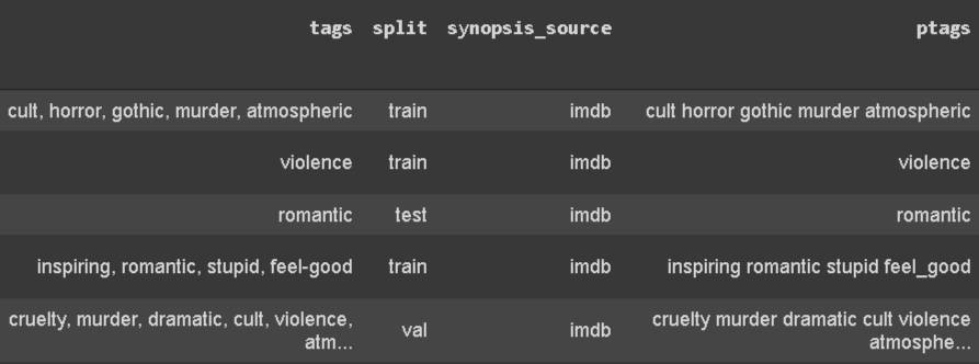
- tags: Tags are labeled tags for a movie. It may take multiple values for a single movie. This will be our prediction label. If we take a closer look, a single tag may have space or a ‘-’. We want our tags to be similar form and thus we will replace whitespace and a dash with an underscore (‘_’). Also, we will separate tags by space instead of the comma. Below is how it looks:
2. Check for missing and duplicate data
Fortunately, there is no missing text in any of the columns but there is for sure, duplicate data in the dataset.
As discussed earlier, if an ‘imdb_id’ column has duplicate, then data must be duplicate. But here, there are few data-points where ‘imdb_id’ is different but the content for ‘title’, ‘plot_synopsis’, and ‘synopsis_source’ are the same. Take a look at below image:

We will be removing such duplicate points with below code:
The above code will remove all duplicate rows which have the same ‘title’,’plot_synopsis’, and ‘ptags’ excluding the first record.
3. Exploring data
3.1 Tags Per Movie
As discussed earlier, a movie may consist of more than one tag and this will be interesting information to look into.
sns.countplot(tags_count)
plt.title(“Number of tags in the synopsis “)
plt.xlabel(“Number of Tags”)
plt.ylabel(“Number of synopsis”)
plt.show()
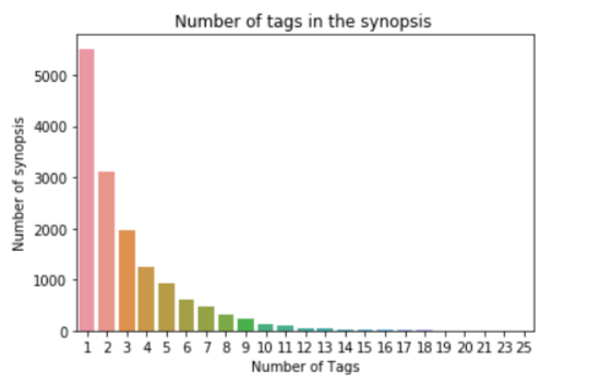
There are 5516 movies which contain only one tag and 1 movie which is labelled for 25 tags.
3.2 Tags frequency analysis
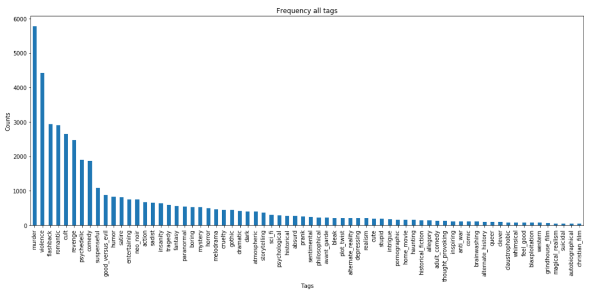
It will be a good idea to analyse tag frequencies to know about frequent and rare tags. Here we can conclude that “murder” is the most frequent tag (5782 occurrences) while “christian film” is the least frequent tag (42 occurrences).
sorted_freq_df.head(-1).plot(kind=’bar’, figsize=(16,7), legend=False)
i=np.arange(71)
plt.title(‘Frequency of all tags’)
plt.xlabel(‘Tags’)
plt.ylabel(‘Counts’)
plt.show()
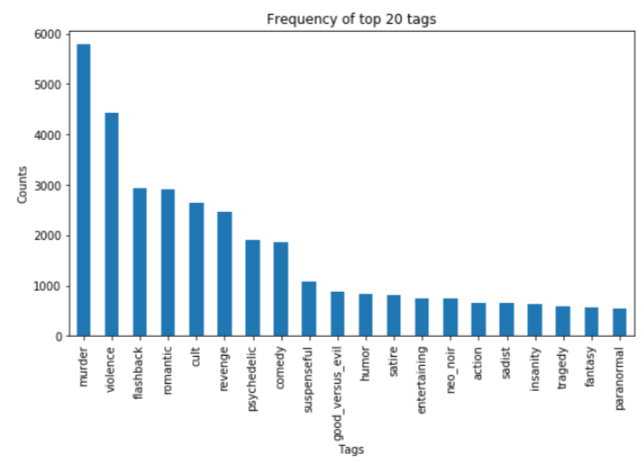
If we consider only the top 20 tags, below is how it looks like:
3.3 WordCloud for tags
Creating a word cloud of a plot synopsis text for a particular tag will help us to understand about the most frequent words for that tag. We will create a word cloud for a murder tag.
# Creating a column to indicate whether a murder tag exists or nor for a movie
data[‘ptags_murder’]= [1 if ‘murder’ in tgs.split() else 0 for tgs in data.ptags]
# creating a corpus for movies with murder tag
murder_word_cloud=”
for plot in data[data[‘ptags_murder’]==1].plot_synopsis:
murder_word_cloud = plot + ‘ ‘
from wordcloud import WordCloud
#building a wordcloud
wordcloud = WordCloud(width=800, height=800, collocations=False,
background_color=’white’).generate(murder_word_cloud)
plt.figure(figsize=(10,10))
plt.imshow(wordcloud)
plt.title(“Words in plots for movies with murder tag”)
plt.axis(“off”)
plt.show()
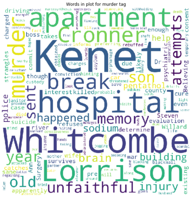
Here we can see words like murder, police, attempts, charged, etc do have a connection with a tag murder semantically. We can do such analysis for all the tags but as we require to cover a lot of other stuff, it won’t be a good idea to increase the length of a blog including all those tag analysis.
4. Text pre-processing
Text in a raw format does have things like HTML tags, special characters, etc, which need to be removed before using text to build a machine learning model. Below is the procedure I used for text processing.
- Removing HTML tags
- Removing special characters like #, _ , -, etc
- Converting text to lower case
- Removing stop words
- Stemming operation
## function to remove html tags
def striphtml(data):
cleanr = re.compile(‘<.*?>’)
cleantext = re.sub(cleanr, ‘ ‘, str(data))
return cleantext
stop_words = set(stopwords.words(‘english’))
stemmer = SnowballStemmer(“english”)
## function to pre-process the text
def text_preprocess(syn_text):
syn_processed = striphtml(syn_text.encode(‘utf-8′)) # html tags removed
syn_processed=re.sub(r'[^A-Za-z]+’,’ ‘,syn_processed) # removing special characters
words=word_tokenize(str(syn_processed.lower())) # device into words and convert into lower
#syn_processed=’ ‘.join(str(stemmer.stem(j)) for j in words if j not in stop_words and len(j)!=1) #Removing stopwords and joining into sentence
return syn_processed
5. Train, validation, and test split
This is fairly simple as splitting strategy is already mentioned in the dataset itself.
val = data[data[‘split’]==’val’]
test = data[data[‘split’]==’test’]
6. Featurization of text
We can use multiple text featurization techniques such as a bag of words with n-grams, TFIDF with n-grams, Word2vec (average and weighted), Sentic Phrase, TextBlob, LDA topic Modelling, NLP/text-based features, etc.
An additional resource to learn about text featurization
For simplicity, I have used TFIDF with 1,2,3-grams featurization which gives pretty good result in fact.
x_train = vectorizer.fit_transform(train[‘processed_plot’])
x_val = vectorizer.transform(val[‘processed_plot’])
x_test = vectorizer.transform(test[‘processed_plot’])
TFIDF with (1,3) grams generated less than 7 million features. Below 2 resources will help you to learn more about TFIDF:
- https://scikit-learn.org/stable/modules/generated/sklearn.feature_extraction.text.TfidfVectorizer.html
- https://www.onely.com/blog/what-is-tf-idf/
7. Machine learning modelling
Before jumping to modelling, let’s discuss the evaluation metrics. Choosing an evaluation metrics is the most essential task as it is a bit tricky depending on the task objective.
Our problem is a multi-label classification problem where there may be multiple labels for a single data-point. We want our model to predict the right categories as much as it can while avoiding the wrong prediction. The accuracy is not a so good metric for this task. For this task, the micro averaged F1 score is the better metric.
Micro averaged F1 score:
F1-Score is derived from recall and precision values. To calculate micro F1 score, we need to calculate micro averaged precision and recall, hence:
Let’s understand how to calculate micro averaged precision and recall from an example. let’s say for a set of data, the system’s
False positive (FP1)=9
False negative (FN1)=3
Then precision (P1) and recall (R1) will be 57.14 and 80 and for a different set of data, the system is
False positive (FP2)=23
False negative (FN2)=9
Then precision (P2) and recall (R2) will be 68.49 and 84.75
Now, the average precision and recall of the system using the Micro-average method is
Micro-average of recall = (TP1+TP2)/(TP1+TP2+FN1+FN2) = (12+50)/(12+50+3+9) = 83.78
The above explanation is borrowed from this brilliant blog.
One more thing before jumping to modeling.
Let’s look into a research paper by dataset publisher which I have already mentioned (a link to paper) in the beginning. They used a micro F1 score along with tag recall and tag learned as evaluation metrics. Below is the snap of their result:
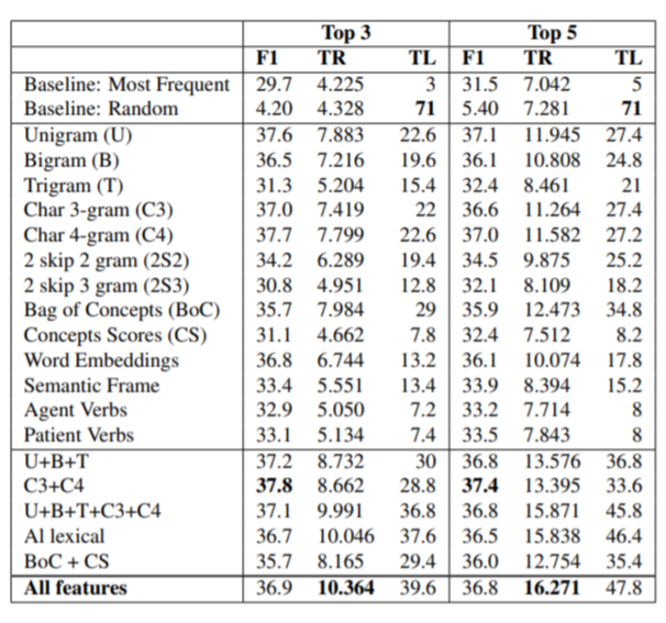
The maximum F1-micro in the list is 37.8. Let’s see how much we would be able to get with a simple model.
To solve a multi-label classification problem, we would use the OneVsRest classifier which at a time classifies one class iteratively. Learn more here.
I have tried with support vector machine and logistic regression. Logistic regression turns out to be a better option.
classifier.fit(x_train, y_train)
predictions = classifier.predict(x_test)print(“micro f1 score :”,metrics.f1_score(y_test, predictions, average = ‘micro’))
print(“hamming loss :”,metrics.hamming_loss(y_test,predictions))—–output—–micro f1 score : 0.34867686650469504
hamming loss : 0.04710189661231041
We got pretty good micro-F1 (0.349 vs 0.378, best result mentioned in the paper) with the LR model.
The final trick!
Precision and recall depend upon TP, FP, TN, and FN. All these metrics depend on predictions (0 or 1) but not on the probability of a prediction.
What if we figure out a way to use probability and check whether it improves micro F1 score or not. To do so, we will use the fact that the default threshold for prediction is 0.5. That simply means we assign 1 if prediction probability is 0.5 or above and 0 otherwise.
Here we will try different threshold values to learn a threshold that maximizes the micro-F1 score.
Let’s try with 0.20 to 0.30 as threshold values.
yhat_val_prob= classifier.predict_proba(x_val)
for t in list(range(20, 31, 1)):
print(t*0.01)
pred_lb=np.asarray(yhat_val_prob>t*0.01, dtype=’int8′)
print(“micro f1 scoore :”,metrics.f1_score(y_val, pred_lb, average = ‘micro’))
—–output—–
0.2
micro f1 scoore : 0.37533010563380287
0.21
micro f1 scoore : 0.3761086785674189
0.22
micro f1 scoore : 0.3761457378551788
0.23
micro f1 scoore : 0.37720425084666587
0.24
micro f1 scoore : 0.3766496254904292
0.25
micro f1 scoore : 0.3773150950248154
0.26
micro f1 scoore : 0.378451509747248
0.27
micro f1 scoore : 0.3784528656435954
0.28
micro f1 scoore : 0.37878787878787873
0.29
micro f1 scoore : 0.377741831122614
0.3
micro f1 scoore : 0.3768382352941177
From above, we can see that using 0.28 as a threshold value we can get the best micro F1 score around 0.379 on the validation dataset.
Let’s see what result the same threshold can give for test data set.
pred_lb=np.asarray(yhat_test_prob>0.28, dtype=’int8′)
print(“micro f1 score :”,metrics.f1_score(y_test, pred_lb, average = ‘micro’))
print(“hamming loss :”,metrics.hamming_loss(y_test,pred_lb))
—–output—–
micro f1 score : 0.3737731458059294
hamming loss : 0.05899764066633302
Here, we improved results on test data from 0.349 to 0.374 just by adjusting threshold values.
We can improve the result by using fewer tags, more data, or complex NLP techniques.
Advantages of keyword extraction:
1. Document Summarization: By extracting keywords, you can quickly identify the most important terms and phrases within a document. These keywords can then be used to generate a concise summary of the document, saving time and effort for users.
2. Information Retrieval: Keywords play a crucial role in search engines and information retrieval systems. Extracting and indexing keywords from documents can enhance search accuracy and improve the relevance of search results.
3. Text Categorization and Classification: Keywords can assist in categorizing and classifying documents by identifying the main themes and topics they cover. This can be particularly helpful in organizing large volumes of textual data or in building recommendation systems.
4. Data Visualization and Exploration: Extracted keywords can be used for visualizing and exploring textual data. Analyzing the distribution of keywords can provide insights into patterns, trends, and relationships among different documents or within a single document.
5. Content Generation and SEO: Identifying relevant keywords is crucial for creating search engine optimized (SEO) content. By extracting keywords related to a specific topic or domain, you can ensure that your content aligns with the target audience’s search intent, increasing visibility and improving search engine rankings.
6. Text Mining and Data Analysis: Keyword extraction is an essential step in text mining and data analysis tasks. It helps identify key features and patterns within a large corpus of documents, enabling more efficient and effective analysis.
7. Information Extraction: Keyword extraction can be used as a preliminary step in more advanced information extraction techniques. By identifying important keywords, it becomes easier to extract specific entities, relationships, or attributes from textual data.
Overall, keyword extraction provides a valuable way to automatically identify and extract meaningful information from text, improving information retrieval, summarization, categorization, and analysis tasks.


